The Koch snowflake

Alejandro Morales & Ana Ernst

Centre for Crop Systems Analysis - Wageningen University

TL;DR
Define parameter for graph nodes
Define methods for VirtualPlantLab.feed! functions
Create Scenes
Visualization of 'Graph' with render()

In this example, we create a Koch snowflake, which is one of the earliest fractals to be described. The Koch snowflake is a closed curve composed on multiple of segments of different lengths. Starting with an equilateral triangle, each segment in the snowflake is replaced by four segments of smaller length arrange in a specific manner. Graphically, the first four iterations of the Koch snowflake construction process result in the following figures (the green segments are shown as guides but they are not part of the snowflake):

$First four iterations fo Koch snowflake fractal$

In order to implement the construction process of a Koch snowflake in VPL we need to understand how a 3D structure can be generated from a graph of nodes. VPL uses a procedural approach to generate of structure based on the concept of turtle graphics.

The idea behind this approach is to imagine a turtle located in space with a particular position and orientation. The turtle then starts consuming the different nodes in the graph (following its topological structure) and generates 3D structures as defined by the user for each type of node. The consumption of a node may also include instructions to move and/or rotate the turtle, which allows to alter the relative position of the different 3D structures described by a graph.

The construction process of the Koch snowflake in VPL could then be represented by the following axiom and rewriting rule:

axiom: E(L) + RU(120) + E(L) + RU(120) + E(L) rule: E(L) → E(L/3) + RU(-60) + E(L/3) + RU(120) + E(L/3) + RU(-60) + E(L/3)

Where E represent and edge of a given length (given in parenthesis) and RU represents a rotation of the turtle around the upward axis, with angle of rotation given in parenthesis in hexadecimal degrees. The rule can be visualized as follows:

Koch construction rule

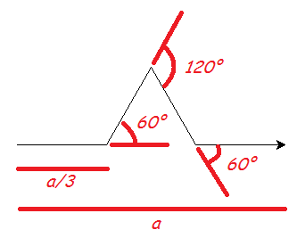
Note that VPL already provides several classes for common turtle movements and rotations, so our implementation of the Koch snowflake only needs to define a class to implement the edges of the snowflake. This can be achieved as follows:

using VirtualPlantLab
import GLMakie ## Import rather than "using" to avoid masking Mesh
using ColorTypes ## To define colors for the rendering
module sn
    import VirtualPlantLab
    struct E <: VirtualPlantLab.Node
        length::Float64
    end
end
import .sn

Note that nodes of type E need to keep track of the length as illustrated in the above. The axiom is straightforward:

const L = 1.0
axiom = sn.E(L) + VirtualPlantLab.RU(120.0) + sn.E(L) + VirtualPlantLab.RU(120.0) + sn.E(L)

The rule is also straightforward to implement as all the nodes of type E will be replaced in each iteration. However, we need to ensure that the length of the new edges is a calculated from the length of the edge being replaced. In order to extract the data stored in the node being replaced we can simply use the function data. In this case, the replacement function is defined and then added to the rule. This can make the code more readable but helps debugging and testing the replacement function.

function Kochsnowflake(x)
    L = data(x).length
    sn.E(L/3) + RU(-60.0) + sn.E(L/3) + RU(120.0) + sn.E(L/3) + RU(-60.0) + sn.E(L/3)
end
rule = Rule(sn.E, rhs = Kochsnowflake)

The model is then created by constructing the graph

Koch = Graph(axiom = axiom, rules = Tuple(rule))

In order to be able to generate a 3D structure we need to define a method for the function VirtualPlantLab.feed! (notice the need to prefix it with VirtualPlantLab. as we are going to define a method for this function). The method needs to two take two arguments, the first one is always an object of type Turtle and the second is an object of the type for which the method is defined (in this case, E).

The body of the method should generate the 3D structures using the geometry primitives provided by VPL and feed them to the turtle that is being passed to the method as first argument. In this case, we are going to represent the edges of the Koch snowflakes with cylinders, which can be generated with the HollowCylinder! function from VirtualPlantLab. Note that the feed! should return nothing, the turtle will be modified in place (hence the use of ! at the end of the function as customary in the VPL community).

In order to render the geometry, we need assign a color (i.e., any type of color support by the package ColorTypes.jl). In this case, we just feed a basic RGB color defined by the proportion of red, green and blue. To make the figures more appealing, we can assign random values to each channel of the color to generate random colors.

function VirtualPlantLab.feed!(turtle::Turtle, e::sn.E, vars)
    HollowCylinder!(turtle, length = e.length, width = e.length/10,
                    height = e.length/10, move = true,
                    colors = RGB(rand(), rand(), rand()))
    return nothing
end

Note that the argument move = true indicates that the turtle should move forward as the cylinder is generated a distance equal to the length of the cylinder. Also, the feed! method has a third argument called vars. This gives acess to the shared variables stored within the graph (such that they can be accessed by any node). In this case, we are not using this argument.

After defining the method, we can now call the function render on the graph to generate a 3D interactive image of the Koch snowflake in the current state

sc = Mesh(Koch)
render(sc, axes = false)

This renders the initial triangle of the construction procedure of the Koch snowflake. Let's execute the rules once to verify that we get the 2nd iteration (check the figure at the beginning of this document):

rewrite!(Koch)
render(Mesh(Koch), axes = false)

And two more times

for i in 1:3
    rewrite!(Koch)
end
render(Mesh(Koch), axes = false)

Other snowflake fractals

To demonstrate the power of this approach, let's create an alternative snowflake. We will simply invert the rotations of the turtle in the rewriting rule

function Kochsnowflake2(x)
   L = data(x).length
   sn.E(L/3) + RU(60.0) + sn.E(L/3) + RU(-120.0) + sn.E(L/3) + RU(60.0) + sn.E(L/3)
end
rule2 = Rule(sn.E, rhs = Kochsnowflake2)
Koch2 = Graph(axiom = axiom, rules = Tuple(rule2))

The axiom is the same, but now the edges added by the rule will generate the edges towards the inside of the initial triangle. Let's execute the first three iterations and render the results First iteration

rewrite!(Koch2)
render(Mesh(Koch2), axes = false)

Second iteration

rewrite!(Koch2)
render(Mesh(Koch2), axes = false)

Third iteration

rewrite!(Koch2)
render(Mesh(Koch2), axes = false)

This is know as Koch antisnowflake. We could also easily generate a Cesàro fractal by also changing the axiom:

axiomCesaro = sn.E(L) + RU(90.0) + sn.E(L) + RU(90.0) + sn.E(L) + RU(90.0) + sn.E(L)
Cesaro = Graph(axiom = axiomCesaro, rules = (rule2,))
render(Mesh(Cesaro), axes = false)

And, as before, let's go through the first three iterations First iteration

rewrite!(Cesaro)
render(Mesh(Cesaro), axes = false)

Second iteration

rewrite!(Cesaro)
render(Mesh(Cesaro), axes = false)

Third iteration

rewrite!(Cesaro)
render(Mesh(Cesaro), axes = false)

This page was generated using Literate.jl.